Six figures putting all three models on one pair of axes, plus the scripts that build them. The study is written up in SUMMARY.md, which reads them in order; the per-question detail behind them is in QUESTIONS.md. Both also exist as self-contained HTML — SUMMARY.html and QUESTIONS.html, with the figures embedded and nothing to resolve — rebuilt by uv run python results-single/build_html.py.
The corpus itself is benchmarks-single/, whose README describes the twelve records. This study is the floor: one condition, no ablation, no cross-graph join. Its job is to make the cross-graph and ontology studies readable, by establishing that a failure there is a failure at what those corpora add.
| Figure | Shows |
|---|---|
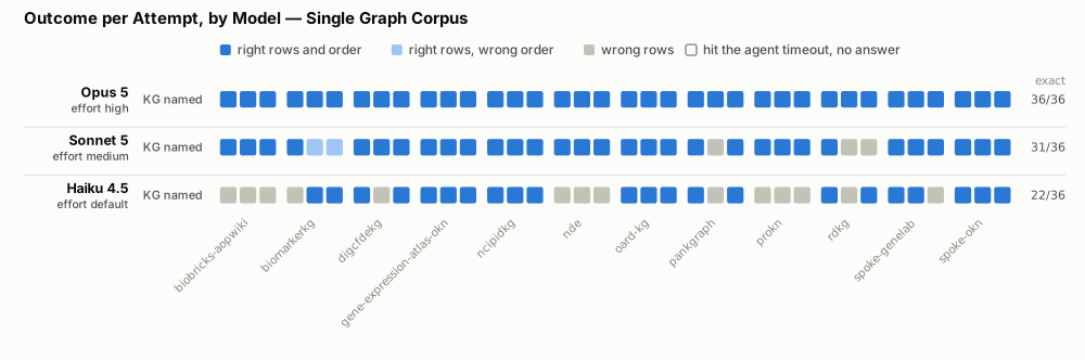
outcome-by-model.svg | what each attempt produced — right rows and order, right rows in the wrong order, wrong rows, or nothing |
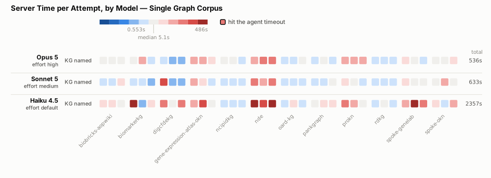
server-time-by-model.svg | seconds each attempt spent inside the server under test |
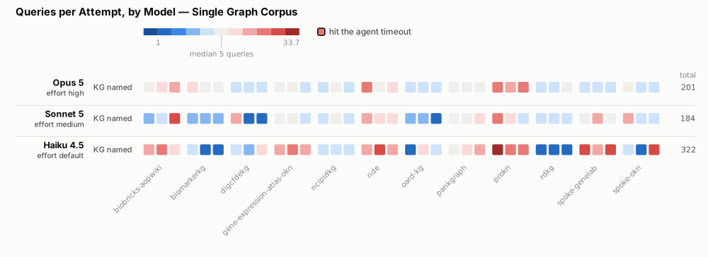
queries-by-model.svg | how many queries each attempt ran |
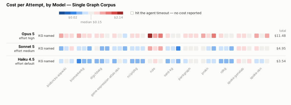
cost-by-model.svg | what each attempt cost, in US dollars |
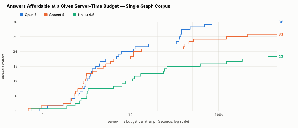
budget-by-server-time.svg | how many answers each model could still afford at a given endpoint budget |
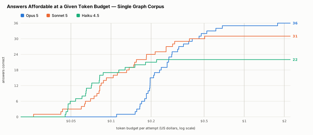
budget-by-cost.svg | the same, with tokens as the scarce resource |
The first four share one layout, so any two can be compared square for square. The two budget figures are a different idiom and are described below.
Rows are the three models, one band each, labeled with the reasoning effort it ran at underneath its name. Unlike the cross-graph study, there is no second level to the banding: this corpus has a single condition — the full toolkit with the graph named — so each model contributes one row rather than three.
Columns are the twelve questions, three squares each: one per attempt, left to right.
Shading on the three quantitative figures is logarithmic and diverging about the median attempt: blue is below typical, red above. The neutral midpoint is the median of the whole figure and the legend states its value. This encodes deviation rather than raw magnitude, which is what makes an outlier visible; the ramp's two ends still carry their absolute values.
A heavy outline would mark an attempt killed at the 900s agent deadline — but no attempt in this corpus hit it, so no square here carries one and no row total is marked ≥. That is worth noticing rather than skipping past: every timing in this study is a completed measurement, unlike the ontology sweep, where two attempts were killed mid-flight and their totals understate.
Two Haiku attempts nevertheless produced no answer, on biomarkerkg and nde. They are drawn as wrong rows, not hollow: the hollow state is reserved for the deadline, because an episode killed mid-flight never reached a verdict, while an agent that finishes and submits nothing has.
The right-hand column totals each row over all 36 of its attempts. On outcome-by-model it is a tally of exact attempts instead — 36/36, 31/36, 22/36.
Every square has a tooltip naming the model, question and value.
outcome-by-model is the one figure to read if you read only one. Opus's row is solid blue; Haiku's is a third gray, with three questions gray across all three attempts. The pale blue squares in Sonnet's row are right rows, wrong order — the data correct and the sort not, on questions whose prose states the sort explicitly. Keeping that state separate from wrong rows is the whole reason the legend has four entries and not two.
The row totals here are sums over all 36 attempts of a model. The Server and Queries columns in each root's generated README.md are one pass — the per-question mean summed over twelve questions — so they are roughly a third of these. Neither is wrong; they answer different questions. Do not put them in the same table.
The grids put one square per attempt, which cannot show a sweep: a budget is a continuous axis, not a condition. The two budget-by-* figures are that other view. Each line steps up once per correct answer, ordered by what that answer cost, and flattens at the model's uncapped total — so a point reads at this budget per attempt, this model would still have got this many right. The curve is exact at every budget, where §7 of SUMMARY.md tabulates four.
There are two because there are two scarce resources, and this corpus is where they disagree most sharply. Under a server-time budget the models keep their uncapped ranking (with a small braid below 6.8 seconds). Under a token budget the ordering inverts outright: at ≤$0.10 Opus scores zero and Haiku scores 17, because every one of Opus's 36 correct answers cost more than a dime. A perfect score is worth nothing when tokens are the scarce resource.
Because this corpus has one condition, these are single-axis curves rather than the small multiples the cross-graph study needs — there is no arm dimension to split on.
Each figure exists as .svg and .png. The SVG is the source of truth — sharper at any zoom, a fifth of the size, and what build_comparison.py writes. The PNGs are rendered from it at 2× (2000px wide) for venues that will not take SVG: manuscript submission, Word, PowerPoint. SUMMARY.md links the PNGs so it stays portable into those tools; the table above links the SVGs.
All six are hand-built. The harness renders one runs root at a time and cannot draw three models on one pair of axes, so nothing regenerates them automatically:
uv run python results-single/build_comparison.pyThe script reads the three roots directly and writes all six figures. To refresh the PNGs afterwards:
./results-single/build_png.shIt renders each SVG through headless Chrome — the same engine the figures were designed against — so the PNG shows what a reader sees in the browser. Set SCALE=3 for a higher-DPI render. Re-run it after any run, rescore or report that changes a root, or the figures will quietly disagree with the tables they sit beside.
It shares its palette, ramp, layout and timeout conventions with the harness's own figure code (src/okn_benchmark/figure.py), which is what keeps a comparison figure readable straight after a per-root one — and what keeps this study's figures readable straight after the other two corpora's.
build_budget.pyRe-reads the recorded episodes under a resource budget and writes the §7 tables to stdout as markdown. It needs no model, no endpoint and no network: the budgets are applied to runs that already exist, so an episode counts only if it was correct and stayed inside the cap.
uv run python results-single/build_budget.py
It refuses to print if any correct episode is missing its recorded cost. The section's claim that these numbers are not lower bounds rests on timeout-killed episodes producing no answer and so never entering a numerator; a silent hole would look exactly like a result.
The tables here are model × budget with no arm dimension, because this corpus has a single condition — which is what makes it the cleanest place in the study to read the effect, since nothing else varies. The computation lives in okn_benchmark.budget and is tested; this script only declares the table shape.